


Updated on 9/28/2019
Data binning is a basic skill that a knowledge worker or data scientist must have. When we want to study patterns collectively rather than individually, individual values need to be categorized into a number of groups beforehand. We can group values by a range of values, by percentiles and by data clustering.
Grouping by a range of values is referred to as data binning or bucketing in data science, i.e., categorizing a number of continuous values into a smaller number of bins (buckets). Each bucket defines an interval. A category name is assigned each bucket. An example of this is the grading system in the U.S. where a $90%$ grade or better is an A, 80–89% is B, etc. The intervals can be set to either equal-width or varying-width. For instance, the 5-point Likert data can be converted into categories with 4 and 5 being “High”, 3 being “Medium”, and 1 and 2 being “Low”.
This post shows two examples of data binning in R and plot the bins in a bar chart as well. The first one uses R Base function cut. The second one uses the data manipulation functions in the dplyr package.
The cut function: Categorizing Continuous Values into Groups
The example is categorizing mean education level per house which was originally measured by numeric values ranged from 0 until 19, perform data binning to place each value into one bucket if the value falls into the interval that the bucket covers.
Data
The dataset contains 32038 observations for mean education level per house. Load the data into R.
library(tidyverse)
data <- read_delim(file = "../data/zipIncome.csv", delim = ',')
v <- data %>% select(MeanEducation,MeanHouseholdIncome) #pick the variable
Run summary with v to find the range of mean education:
summary(v)## MeanEducation MeanHouseholdIncome
## Min. : 0.00 Min. : 0
## 1st Qu.:11.88 1st Qu.: 37644
## Median :12.43 Median : 44163
## Mean :12.52 Mean : 48245
## 3rd Qu.:13.10 3rd Qu.: 54373
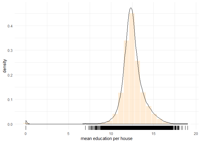
## Max. :19.00 Max. :250000The summary shows the range, \([0,19]\). The median education level per house is \(12.43\), to the left of, but very close to the mean. The frequency chart with a density curve shows a bell-shaped distribution with a dense area between 10 and 16.
ggplot(data = v, mapping = aes(x=MeanEducation)) +
  geom_histogram(aes(y=..density..),fill="bisque",color="white",alpha=0.7) +
  geom_density() +
  geom_rug() +
  labs(x='mean education per house') +
  theme_minimal()
data binning plot
While the density curve is informative, it can be too technical for average users to read. In this case, a better way is binning the values into discrete categories and plotting the count of each bin in bars.
Defining breaks and cut a vector into bins
# set up cut-off values
breaks <- c(0,2,4,6,8,10,12,14,16,18,20)
# specify interval/bin labels
tags <- c("[0-2)","[2-4)", "[4-6)", "[6-8)", "[8-10)", "[10-12)","[12-14)", "[14-16)","[16-18)", "[18-20)")
# bucketing values into bins
group_tags <- cut(v$MeanEducation,
                  breaks=breaks,
                  include.lowest=TRUE,
                  right=FALSE,
                  labels=tags)
# inspect bins
summary(group_tags)
## [0-2) [2-4) [4-6) [6-8) [8-10) [10-12) [12-14) [14-16) [16-18)
## 120 0 0 24 330 9067 19075 3115 294
## [18-20)
## 13The code chunk above produces a factor group_tags which maps each original education value into one of the eleven bins. Each level is named by a string in the vector labels. Each value in bins indicates the interval a value falls into. The summary of group_tags lists the count in each bin.
cut by default outputs an unordered factor. To get an ordered factor, rebuild the factor from group_tags:
education_groups <- factor(group_tags,
                           levels = labels,
                           ordered = TRUE)
Bar Chart
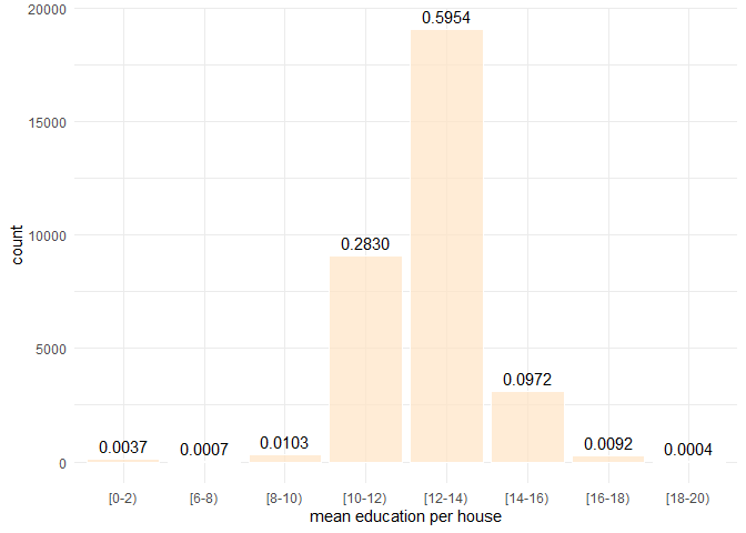
Plot the bins:
ggplot(data = as_tibble(group_tags), mapping = aes(x=value)) +
  geom_bar(fill="bisque",color="white",alpha=0.7) +
  stat_count(geom="text", aes(label=sprintf("%.4f",..count../length(group_tags))), vjust=-0.5) +
  labs(x='mean education per house') +
theme_minimal() 
data binning plot
Categorizing by the dplyr Functions
Define bucket intervals and give names
tags <- c("[0-2)","[2-4)", "[4-6)", "[6-8)", "[8-10)", "[10-12)","[12-14)", "[14-16)","[16-18)", "[18-20)")Place mean education levels into buckets. Store groups as a new column.
v <- data %>% select(MeanEducation,MeanHouseholdIncome) #pick the variable
vgroup <- as_tibble(v) %>%
  mutate(tag = case_when(
    MeanEducation < 2 ~ tags[1],
    MeanEducation >= 2 & MeanEducation < 4 ~ tags[2],
    MeanEducation >= 4 & MeanEducation < 6 ~ tags[3],
    MeanEducation >= 6 & MeanEducation < 8 ~ tags[4],
    MeanEducation >= 8 & MeanEducation < 10 ~ tags[5],
    MeanEducation >= 10 & MeanEducation < 12 ~ tags[6],
    MeanEducation >= 12 & MeanEducation < 14 ~ tags[7],
    MeanEducation >= 14 & MeanEducation < 16 ~ tags[8],
    MeanEducation >= 16 & MeanEducation < 18 ~ tags[9],
    MeanEducation >= 18 & MeanEducation < 20 ~ tags[10]
    ))
summary(vgroup)
## MeanEducation MeanHouseholdIncome tag
## Min. : 0.00 Min. : 0 Length:32038
## 1st Qu.:11.88 1st Qu.: 37644 Class :character
## Median :12.43 Median : 44163 Mode :character
## Mean :12.52 Mean : 48245
## 3rd Qu.:13.10 3rd Qu.: 54373
## Max. :19.00 Max. :250000The new column tag from case_when is a character vector. To make it a factor, do;
vgroup$tag <- factor(vgroup$tag,
                       levels = tags,
                       ordered = FALSE)
summary(vgroup$tag)
## [0-2) [2-4) [4-6) [6-8) [8-10) [10-12) [12-14) [14-16) [16-18)
## 120 0 0 24 330 9067 19075 3115 294
## [18-20)
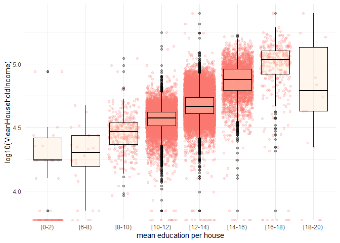
## 13BoxPlot: Distribution of Mean Household Income for Each Level of Education
ggplot(data = vgroup, mapping = aes(x=tag,y=log10(MeanHouseholdIncome))) +
  geom_jitter(aes(color='blue'),alpha=0.2) +
  geom_boxplot(fill="bisque",color="black",alpha=0.3) +
  labs(x='mean education per house') +
  guides(color=FALSE) +
theme_minimal() 
data binning plot
Set up a Python environment for doing Data Science in Jupyter Notebook with Conda virtual environment
Share this post
Twitter
Facebook
LinkedIn
Email