


Predictive learning is a process where a model is trained from known predictors and the model is used to predict, for a given new observation, either a continuous value or a categorical label. This results in two types of data mining techniques, classification for a categorical label and regression for a continuous value.
Linear regression is not only the first type but also the simplest type of regression techniques. As indicated by the name, linear regression computes a linear model which is line of best fit for a set of data points. In a two-dimensional dataset, i.e., two variables, input variable (predictor) \(x\) and output (dependent) variable \(y\), the resulting linear model represents the linear part in the relationship between \(x\) and \(y\), which is expressed in the following equation:
\[ \begin{eqnarray} y \approx ax + b \tag{1} \end{eqnarray} \]
The parameters \(a\) and \(b\) are often calculated by the least squares approach. After developing the model, given a sample value of \(x\), the model can compute its associated \(y\), which, in predictive learning, is considered as the predicted value of true \(y\).
1. Least Squares Approach
With the linear model above, each \(x\) will produce a fitted value \({\hat y}\). The least squares approach finds \(a\) and \(b\) which minimize the sum of the squared distances between each observed response \(y\) to its fitted value \({\hat y}\). The sum of the squared errors over \(n\) data points is
\[ \begin{eqnarray} SE = \sum_{i=1}^n({\hat y_i}-y_i)^2 \\\\\\ = \sum_{i=1}^n(ax_i + b -y_i)^2 \tag{2} \end{eqnarray} \]
To optimize \(SE\) with \(a\) and \(b\), let two following partial derivatives be zero,
\[ \frac{\partial SE}{\partial a} = 0 \\\\\\ \frac{\partial SE}{\partial b} = 0 \]
After simplifying the equations above (the steps are skipped here), it shows that two points are on the best-fit line:
\[ \begin{eqnarray} (\overline{x}, \overline{y}), \left(\frac{\overline{x^2}}{\overline{x}}, \frac {\overline{xy}}{\overline{x}}\right) \end{eqnarray} \]
The overline represents the mean.
Thus, the slope \(a\) and the intercept \(b\) are
\[ a = \frac {\overline{x}\hspace{.1cm}\overline{y}-\overline{xy}} {\left(\overline{x}\right)^2-\overline{x^2}} \\\\\\ b = {\overline{y}}-a{\overline{x}} \tag{3} \]
Multiple predictor variables
If the predictor consists of \(m\) variables, \(x_1, x_2, ..., x_m\), then the linear equation for the response \(y\) is
\[ \begin{eqnarray} y \approx b + \sum_{i=1}^{m}a_ix_i \tag{4} \end{eqnarray} \]
2. R-squared
To measure how good a linear regression line is, R-squared, a.k.a. the coefficient of determination, is the percentage of variation in \(y\) which is captured by the linear model. R-squared is calculated by the following formula:
\[ \begin{eqnarray} r^2 &=& 1- \frac{SE}{SE_{\overline{y}}} \\\\\\ &=& 1 - \frac { \sum_{i=1}^n({\hat y_i}-y_i)^2 } { \sum_{i=1}^n(\overline{y}-y_i)^2 } \tag{5} \end{eqnarray} \]
R-squared is between 0 and 1. In general, the higher R-squared, the better the model fits the data.
3. R Function lm
R has a function lm to fit a linear model. The function lm returns an object of class "lm".
Example 1
The following snippet shows an example of using lm to fit a dataset of two variable x and y.
df <- data.frame(x=c(1:50))
df$y <- 2 + 3*df$x + rnorm(50, sd=10)
lm.xy <- lm(y~x, df)
summary(lm.xy)
The following is the result after running the R snippet above.
Call:
lm(formula = y ~ x, data = df)

Residuals:
    Min      1Q  Median      3Q     Max
-22.174  -6.641  -1.059   7.731  24.380

Coefficients:
            Estimate Std. Error t value Pr(>|t|)
(Intercept)  -2.2205     3.2104  -0.692    0.492
x             3.1069     0.1096  28.355   <2e-16 ***
---
Signif. codes:  0 ‘***’ 0.001 ‘**’ 0.01 ‘*’ 0.05 ‘.’ 0.1 ‘ ’ 1

Residual standard error: 11.18 on 48 degrees of freedom
Multiple R-squared:  0.9437,	Adjusted R-squared:  0.9425
F-statistic:   804 on 1 and 48 DF,  p-value: < 2.2e-16
Accessing Results
The developed model is read from Coefficients which is y = -2.2205 + 3.1069x.
To examine a fit, use the following expression to access R-squared in the summary, which is \(0.9436641\).
summary(lm.xy)$r.squared The Residuals are differences between each \(y\) and its fitted value \({\hat y}\).
residuals(lm.xy)To get the coefficients, call the coef function.
coef(lm.xy)

(Intercept)           x
  -2.220484    3.106902
Other information
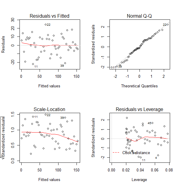
In addition, the lm object lm.xy can be plotted by the following script:
par(mfrow=c(2,2))
plot(lm.xy)
To go back to a single graph per window, run
par(mfrow=c(1,1)).
Example 2 (Multiple predictor variables)
The following snippet shows how to fit a linear model of \(z\) against two predictor variables \(x\) and \(y\).
1df <- data.frame(x=c(1:50))
2df$y <- 2 + 3*df$x + rnorm(50, sd=10)
3df$z <- -2 + 3*df$x -5*df$y + rnorm(50,sd=1)
4
5lm.zxy <- lm(z ~ x+y, df)
6summary(lm.zxy)
Example 3
The following is an example which constructs three response variables \(y1\), \(y2\) and \(y3\) from a predictor variable \(x\) by adding random gaussian noise and compute linear regression model for each as well.
1df <- data.frame(x = c(1:50))
2# y = 2 + 3x + N(0,sd)
3df$y1 <- 2 + 3 * df$x + rnorm(50, sd = 10)
4df$y2 <- 2 + 3 * df$x + rnorm(50, sd = 30)
5df$y3 <- 2 + 3 * df$x + rnorm(50, sd = 50) 1library(ggplot2)
2#install.packages("devtools")
3#library(devtools)
4#install_github("kassambara/easyGgplot2")
5library(easyGgplot2)
6
7# lm_eqn creates a string which writes the linear model equation.
8lm_eqn = function(m) {
9 l <- list(a = format(coef(m)[1], digits = 2),
10 b = format(abs(coef(m)[2]), digits = 2),
11 r2 = format(summary(m)$r.squared, digits = 3));
12 if (coef(m)[2] >= 0) {
13 eq <- substitute(italic(hat(y)) == a + b %.% italic(x)*","~~italic(r)^2~"="~r2,l)
14 } else {
15 eq <- substitute(italic(hat(y)) == a - b %.% italic(x)*","~~italic(r)^2~"="~r2,l)
16 }
17 as.character(as.expression(eq));
18}
19
20# createPlot returns a ggplot object that visualizes each pair x and y in scatterplot with a linear regression line above.
21createPlot <- function(vec,ylabel){
22 p <- ggplot(df, aes(x = df$x, y = vec)) +
23 geom_smooth(method="lm",se=FALSE, color="red", formula=y~x) +
24 geom_point() +
25 labs(x="x",y=ylabel) +
26 theme(panel.background=element_rect(fill='white',colour = "black"),axis.title=element_text(size=9,face='bold'))+
27 geom_text(aes(x = 15, y = max(vec)-20), size=4, label = lm_eqn(lm(vec ~ x, df)), parse = TRUE)
28 return(p)
29}
30
31library(plyr)
32ps <- apply(df[,2:4], 2, createPlot, ylabel='y')
33
34#options(repr.plot.width=5,repr.plot.height=5)
35ggplot2.multiplot(ps[[1]], ps[[2]], ps[[3]], cols=1)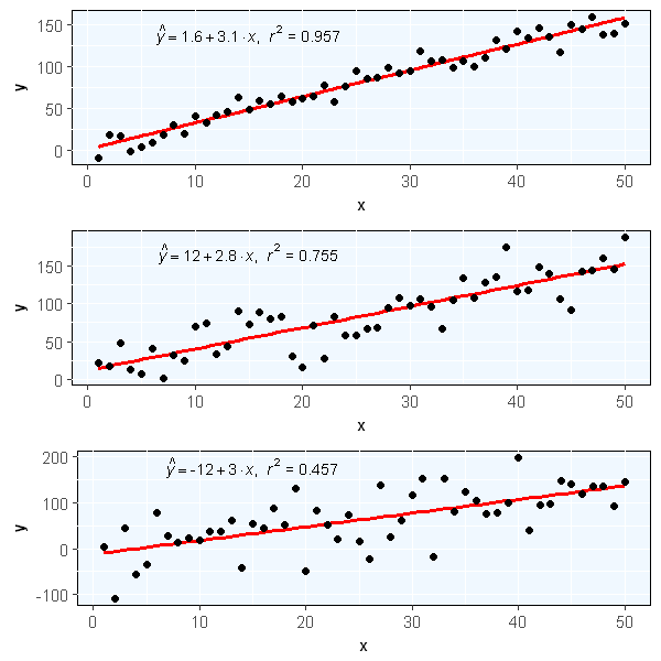
4. Applications
For the prediction purpose, linear regression can
- Fit a linear model for the relationship between a quantitative label \(y\) and one or more predictors (regular attributes). The trained linear model can predict \(y\) for the instances without accompanying \(y\).
For descriptive learning, linear regression can
Measure the strength of the relationship between \(y\) and each predictor attribute,
Identify the less significant predictors.
Continue with the post Predictive Learning from an Operational Perspective
Share this post
Twitter
Facebook
LinkedIn
Email