


Univariate Graphics in R
This post shows some R basic graphics commands for making six types of plots, scatter plot, histogram, boxplot, dot chart, density plot and empirical CDF. A sample R function is given.
This post shows how to use some of R basic graphics techniques and plotting features to explore a single numeric variable.
Create a Custom Function univPlots
The function univPlots takes a numeric vector and creates 6 plots: scatterplot, dotchart, histogram, density plot, CDF (cumulative distribution function) plot and boxplot.
univPlots <- function (x){
        # set up a matrix layout for multiple plots
        mat <- rbind(1:3, 4:6)
        layout(mat)
        # 1
        plot(x, main='scatter plot')
        # 2
        hist(x, main="frequency")
        # 3
        boxplot(x, main='boxplot')
        # 4
        dotchart(x, main='dot chart')
        rug(x)
        # 5
        x.density <- density(x)
        plot(x.density, main="density")
        polygon(x.density, col="lightblue", border="black")
        # 6
        plot(ecdf(x),main='empirical CDF')

	#reset plot layout
	layout(c(1,1))
}
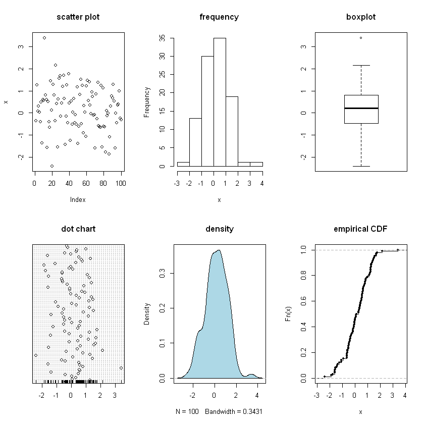
Example 1: random normal distribution
In this example, a sample variable of 100 points is randomly generated from normal distribution with zero mean and unit standard deviation.
# randomly generate 100 points from normal distribution with zero mean and unit sd
x <- rnorm(100, mean=0, sd=1)
# Call univPlots on x
univPlots(x)
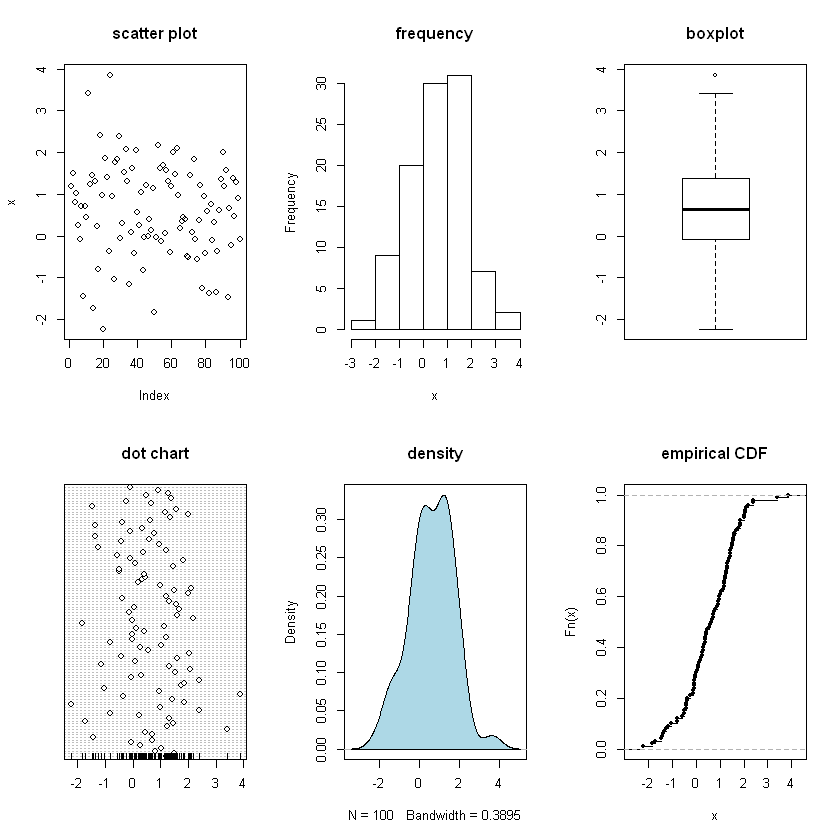
Example 2: noise-added random Normal distribution
In this example, the previous variable x is distorted by adding random Gaussian noise from \(N(0.5,0.5)\)
# randomly generate 100 points from normal distribution with zero mean and unit sd
noise <- rnorm(100, mean=0.5, sd=0.5)
x.distort <- x + noise

univPlots(x.distort)
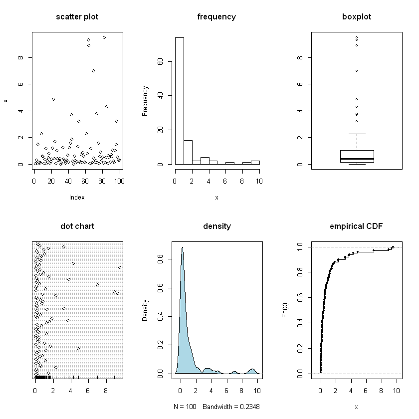
Example 3: random Pareto distribution
Next we plot a random variable of 100 points from a Pareto distribution of location parameter 1 and dispersion parameter 2.
library(rmutil)
x.pareto <- rpareto(100, m=1, s=2)
univPlots(x.pareto)
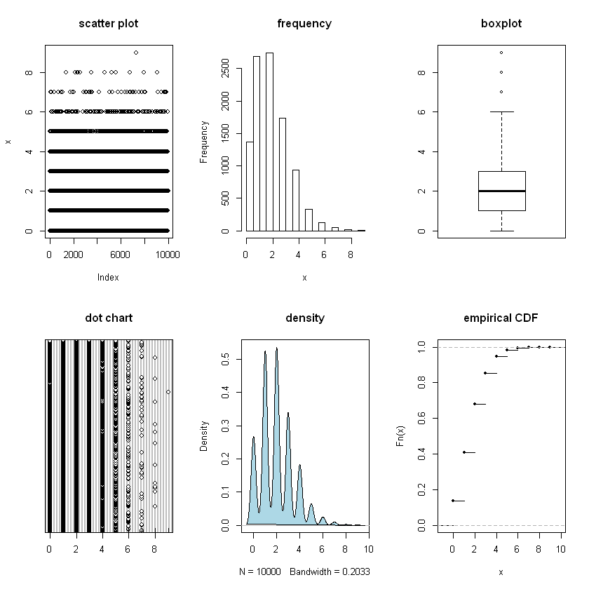
Example 4: random Poisson distribution
This example shows a discrete random variable from Poisson distribution whose expected number of occurrences, \(\lambda\), is 2.
(wikipedia) Poisson distribution expresses the probability of a given number of events occurring in a fixed interval of time and/or space if these events occur with a known average rate and independently of the time since the last event.
x.possion <- rpois(10000, lambda=2)
univPlots(x.possion)
Share this post
Twitter
Facebook
LinkedIn
Email