


This post shows you how to visualize association rules by using the R packages arules and aulesViz. In order to better understand the script, you may have already completed the following parts.
- Part 1 Transactions Class in arules
- Part 2 Read Transaction Data
- Part 3 Generate Itemsets
- Part 4 Generate Rules
The Basket Data
In Part 2 Read Transaction Data, we have read the following five shopping baskets in a plain text file, into transactions of the Transactions class.
 f,a,c,d,g,l,m,p
 a,b,c,f,l,m,o
 b,f,h,j,o
 b,c,k,s,p
a,f,c,e,l,p,m,nwe run arules::apriori with the parameter target set to frequent itemsets. By assigning values to the parameters support, and set minlen and maxlen equal to each other, the apriori function returns all itemsets of a specific length having the minimum support or above.
we run arules::apriori with the parameter target set to rules. By assigning values to the parameters support and confident, and set minlen to prune the rules of 1 item, the apriori function returns all the rules having at least 2 items which exceeds the confident threshold.
In this part, we visualize how these three quality measures are related. Do they tend to change in the same or opposite way?
Visualization 2: Support, Confidence, Lift
Generate Rules
The following script will return to rules, all the rules whose support is at least \(0.1\) and confidence is at least \(0.6\).
#rules having at least a confidence of 0.6
rules <- apriori(
  transactions,
  parameter = list(support=0.1, confidence=0.6, target="rules")
)
For the script details, refer to Part 4 Generate Rules.
A Summary of the Rules
Run the summary with rules.
summary(rules)## set of 1985 rules
##
## rule length distribution (lhs + rhs):sizes
## 1 2 3 4 5 6 7 8
## 7 78 299 554 570 346 115 16
##
## Min. 1st Qu. Median Mean 3rd Qu. Max.
## 1.000 4.000 5.000 4.602 5.000 8.000
##
## summary of quality measures:
## support confidence lift count
## Min. :0.2000 Min. :0.6000 Min. :0.8333 Min. :1.000
## 1st Qu.:0.2000 1st Qu.:1.0000 1st Qu.:1.2500 1st Qu.:1.000
## Median :0.2000 Median :1.0000 Median :1.6667 Median :1.000
## Mean :0.2288 Mean :0.9909 Mean :2.0421 Mean :1.144
## 3rd Qu.:0.2000 3rd Qu.:1.0000 3rd Qu.:1.6667 3rd Qu.:1.000
## Max. :0.8000 Max. :1.0000 Max. :5.0000 Max. :4.000
##
## mining info:
## data ntransactions support confidence
## transactions 5 0.1 0.6The summary shows that
- 1985 rules with a length between 1 and 8 items
- range of support: 0.2 - 0.8
- range of confidence: 0.6 - 1.0
- range of lift: 0.8 - 5
Scatterplot
library(arulesViz)
plot(rules)
## To reduce overplotting, jitter is added! Use jitter = 0 to prevent jitter.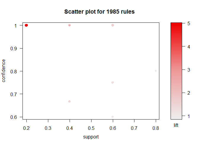
The plot doesn't reveal much information because of the very small dataset having only five transactions. However, it shows that
- With the same support, when lift is high, confidence is high.
- With the same support, When lift is low, confidence doesn't show obvious linear relationship.
We can create the plot for a larger dataset, Groceries from the arules package.
The Groceries Data
data("Groceries")
#
rules <- apriori(
  Groceries,
  parameter = list(support=0.001, confidence=0.6, target="rules")
)
plot(rules)
## To reduce overplotting, jitter is added! Use jitter = 0 to prevent jitter.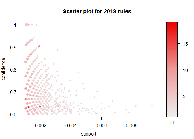
Share this post
Twitter
Facebook
LinkedIn
Email